Transcripción completa del PDF reformateada para lectura web. Descargar PDF original para tablas, figuras y referencias.
• Copyright 2015 Santos, Miguel; and the President and Fellows of Harvard College

Revised on September 2015 Abstract Venezuela is an oil-dependent economy subject to large exogenous shocks, with a rigid labor market. These features go straight at the heart of two weaknesses of real business cycle (RBC) theory widely reported in the literature: Neither shocks are volatile enough nor real salaries are sufficiently flexible as required by the RBC framework to replicate the behavior of the economy. We calibrate a basic RBC model and compare a set of relevant statistics from RBC-simulated time series with actual data for Venezuela and the benchmark case of the United States (1950-2008). In spite of Venezuela being one of the most heavily intervened economies in the world, RBCsimulated series provide a surprisingly good fit when it comes to the non-oil sector of the economy, and in particular for labor markets. Large restrictions on dismissal and widespread minimum (nominal) wage put all the burden of adjustment on prices; which translate into highly volatile real wages. J.E.L. Codes: E10, E32, O47, O54, Q32 Keywords: Macroeconomics, RBC, oil shocks, labor markets, Venezuela. _________________________________
1. Introduction
The theory of business cycles studies the causes leading to and consequences resulting from recurrent expansions and contractions in aggregate economic activity. The idea that a few equations can have the power to replicate means, volatilities, relative volatilities, auto-correlations and crosscorrelations observed in time series of real macroeconomic data is very appealing and has motivated a significant number of authors since the seminal contributions of Kydland and Prescott (1982) and Long and Plosser (1983). Real business cycle theory assumes that these periodic fluctuations are caused primarily by real factors. It has become ever less ambitious and nowadays does not aspire to explain why business cycles exist, but rather to assess and interpret the movements and co-movements of real variables along the cycle.
Most of the empirical evidence in support or denial of RBC models is focused on OECD countries: These are supposed to be fully functioning market economies with appropriate institutional and policy settings. Our purpose here is somewhat the opposite. We set ourselves to study how an RBC model would fare in explaining historical data moments for Venezuela, which throughout the sample period (1950-2008) has been one of most heavily governmentintervened economies, one with a large number of market failures and unsteady political and institutional framework. There have been many papers using RBC models to assess the impacts of oil shocks in oil-importing countries (i.e. Kilian, 2006), but to our knowledge this is the first attempt at
using them to understand the cycles in an oil-exporting country. Our interest has been spurred by a number of economic reasons.
The use of Solow residuals as a proxy for exogenous technology shocks has been a permanent source of criticism for RBC models. The reason is that in order to approximate movements and co-movements of historical data, the RBC needs to be fed with large, persistent and volatile technological shocks. This is unappealing, as emphasized by Summers (1986), since to simulate a recession you would need an implausible degree and frequency of technological regress (negative exogenous technology shocks).
As it turns out, the Venezuelan economy is indeed affected by large, frequent, volatile and exogenous shocks: oil prices. The oil sector of the economy is an enclave that represents an average of 30% of gross domestic product (GDP) 1 and 1.1% of employment, while providing 85% of exports. As the country does not have a stabilization fund and fiscal policy is highly procyclical, oil shocks are transmitted and even amplified to the rest of the (nonoil) economy (see Hausmann, Talvi and Perotti, 1996; Erbil, 2011) becoming the driving force behind the business cycle. As exogenous oil shocks are normally not matched by corresponding variations in capital or labor, they tend to be gathered in the Solow residuals (Finn, 1995).
A second critique made to RBC models has to do with simulated real wages being far too pro-cyclical relative to those observed in real data. King and Rebelo (2000), using quarterly data for the United States for the period (1947- 1996), report that the simulated standard deviation of employment relative to output is roughly half of the observed (0.99 in actual data as compared to simulated 0.48). 2 On the other hand, simulated standard deviation of real wages relative to output is substantially larger than the observed one (0.38 in real data as compared to simulated 0.54). That is to say that, in contrast to observed time series, the RBC model has an internal mechanism of adjustment in the labor market that relies less on quantities (workers) and more on prices (real wages).
The Venezuelan labor market has particular features that make it appealing from a RBC perspective. As widely reported by the World Bank 3 and a number of studies (see for instance Alayon et.al. 2002), throughout history Venezuela had one of the most rigid and distorted labor laws in the world, with high relative firing costs, widespread minimum salary, and more recently, forbidden dismissal below certain salary levels. 4 Within that framework, the market response to shocks in demand has been adjusting real salaries by means of large swings in inflation. Accordingly, the cyclical component of wages is much more volatile and (positively) correlated with output than in the
United States. The flip side of that coin is that, as quantitative labor restrictions prevent the number of workers from adjusting to shocks, employment tends to be much less volatile and correlated with output (less pro-cyclical) than in the United States. As both features (high real wage volatility and low employment volatility) run along the patterns of RBCsimulated time series, the model is able to provide a better match of real historical data, at least from a labor market standpoint.
The paper is organized as follows. Section two provides a complete growth accounting exercise for Venezuela and the benchmark case of the United States for the period 1950-2008. Within Venezuela, we have worked out Solow residuals and derived productivity shocks for both the economy as a whole and for a reduced economy consisting only of the non-oil sector. In section three stylized facts of real business cycle data are presented for both countries (including Venezuela’s non-oil sector). Section four introduces the standard RBC model and derives its equilibrium conditions. Section five is devoted to calibration. I have relied on Venezuela’s Central Bank statistics and Baptista (2011) to calibrate an RBC model for the non-oil sector of the Venezuelan economy, which is then fed by exogenous shocks coming from the oil sector. In section six relevant statistics coming out of the simulation are presented, and in section seven I analyze the potential sources of differences in the performance of the RBC model for both economies. Conclusions and policy recommendations are presented in section eight.
2. Growth Accounting
In order to identify the productivity shocks that will be later input into the RBC model, I have calculated Solow residuals from a standard growth accounting exercise. A Cobb-Douglas aggregate production function has been assumed:
yy tt = aa tt kk tt

where yy tt stands for aggregate output, k t for net non-residential capital stock, n t for labor input , and α is the capital share of output. Taking logs on both sides and clearing out technology ( aa tt ) leads to:

All the data for Venezuela has been taken from the Venezuelan Central Bank and Baptista (2011). Capital stocks have been built using the perpetual inventory method. The average capital share of output used is 43.2% (average for the period 1950-2008), which is not far from the 40% that Gollin (2002)
estimates for Venezuela in his seminal paper on income shares for Latin America. In the case of the United States, data for gross domestic product (GDP) and non-residential capital stock were obtained from the Bureau of Economic Analysis (BEA), whereas data for the labor input comes from the Federal Reserve Bank of St. Louis. The capital share of output used was 0.33, as elsewhere in the literature (see for example Gertler and Karadi, 2011; Sims, 2012; Gertler and Kyiotaki, 2012).
Over the sample period (1950-2008) the income gap between Venezuela and United States widened considerably: Assuming that both countries started at the same place, by 2008 Venezuela income per capita would have been just 44.1% of that of the United States, as reported in Figure 1. 5
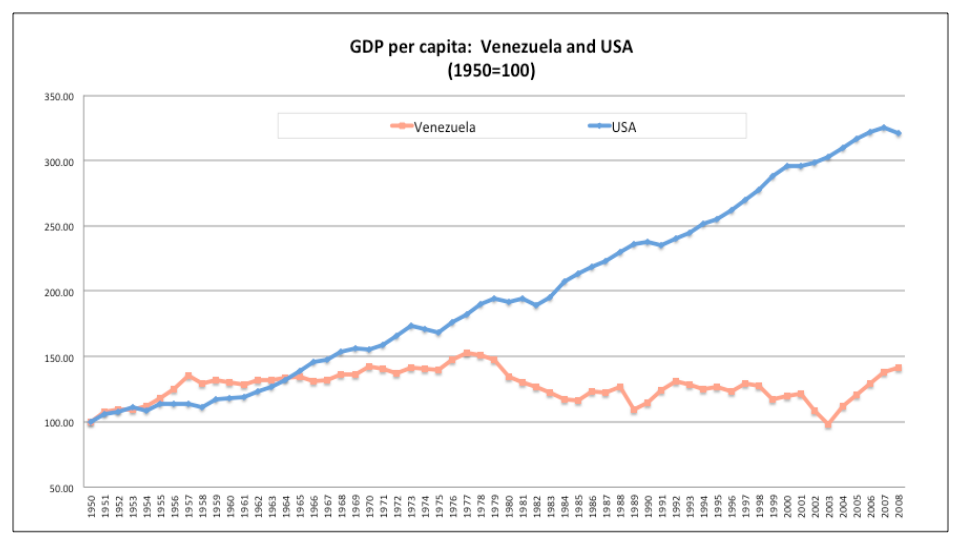
We can differentiate two distinct periods in the evolution of Venezuelan GDP. While GDP per capita expanded 1.1% per year (34.5% in total) in the twenty-seven years spanning between 1950-1977, it collapsed by -0.24% per year (7.2% in total) on the following 31 years (1977-2008). One of the most spectacular cases of economic growth turned into a colossal growth failure.
A growth accounting exercise helps in identifying the sources behind the dismal differences in growth performance in these periods. We have done this exercise using workers, total hours, and hours per worker as a proxy for the labor input. 6 While these methods portray growth evolution from different perspectives, they yield very similar average total factor productivity and almost identical total factor productivity shocks. 7 As we can see from Figure 2, total factor productivity accounts for most of the income gap between the United States and Venezuela. Assuming again that both countries started at same level, by 2008 the difference in income based solely in differential total factor productivity would have been 48%.
These results are in line with those reported for both countries by Cole, Ohanian, Riascos and Schmitz (2005) in their study of Latin America; and also with those estimated by Calcavanti, de Abreu and Veloso (2012) for Venezuela.
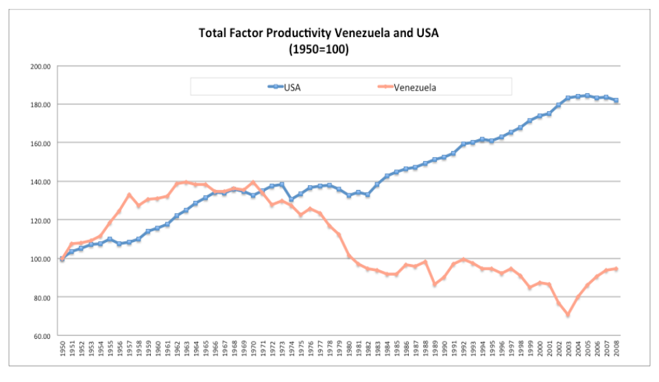
We can see that while Venezuelan GDP per capita peaks in 1977, its total factor productivity reached its crest seven years earlier, around 1970. From there onwards, growth per capita was driven by a large increase in the stock of capital per worker. Those seven years where characterized by a large investment boom, that did not derive its returns from productivity but rather out of a number of market distortions prevalent at the time (appreciated exchange rate, guaranteed demand coming from oil boom, low tax rates).
Table I below contains growth accounting results in total and per hour worked, for both countries and divided into the sub-periods mentioned above.
We can see that from 1950-1977 the contribution of total factor productivity in
Venezuela was lower than in the United States (0.84% vs. 1.21%). Figure 2 provide clues indicating that factor productivity was very similar in both countries over the first twenty years of the sub-sample, the difference originating over last seven years of that period.
Table I
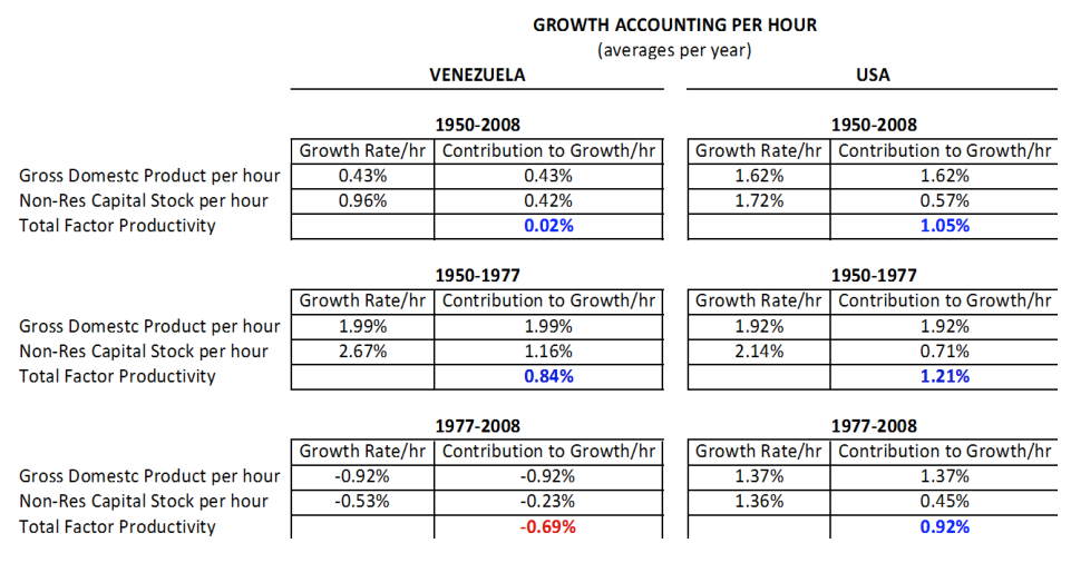
For the second sub-period (1977-2008), the contribution of total factor productivity per hour was not only lower than that of the United States, but significantly negative (-0.69%). Such a loss, coupled with a fall on the stock of non-residential capital per hour worked (-0.23%), lead to an average rate of growth of -0.92%. In these 31 years Venezuela lost 24.9% of its income per unit of labor. Table I also provides enough evidence pointing towards poor total factor productivity being the driving force behind the income gap reported in
Figure 1. These results are consistent with those of Bosworth and Collins
(2008) and Loayza, Fajnzylber, and Calderon (2005).
The distinction between these periods is important because they roughly correspond to two different institutional arrangements as related to the exploitation of oil. Between 1950 and 1970 it was run by private companies, which were awarded concessions over oil fields and heavily taxed. Within this context, the government launched a massive program of investment in public infrastructure and electricity plants that spurred growth and eased productivity in the manufacturing sector. The Yom Kippur war in 1973 and the subsequent oil embargo imposed by Arab countries to the United States had a positive impact in oil prices, feeding the greed of the Venezuelan authorities and paving the way for the nationalization of the industry, which was completed in 1976. From then onwards, the government moved beyond the development of public infrastructure to massive intervention of the economy, gradually substituting the market in the allocation of the oil windfall within the context of state-capitalism policies.
Oil vs. Non-oil Using Venezuelan Central Bank statistics and the revised dataset provided by Baptista (2011) we have disentangled the differences in factor contribution and total factor productivity for the oil and non-oil sectors. The results reported on Table II have been calculated using a slight variation on the
accounting methodology as in Hayashi and Prescott (2002): Growth per worker has been decomposed into the contribution of non-residential capital per worker and average hours per worker (total factor productivities remain the same).
Table II
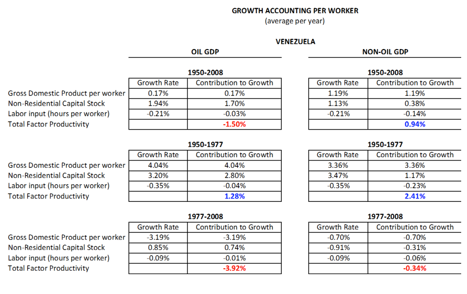
The differences are startling. The non-oil sector of the economy exhibits annual average positive total factor productivity of 0.94% throughout the sample, in stark contrast to the -1.50% exhibited by the oil sector.
Within the period of steep decline in Venezuela’s income (1977-2008), the non-oil sector experienced a loss in GDP per worker of 0.70% per year (19.6% in total). Over the same period, out per worker in the oil industry has fallen an
annual average of 3.19% (a total decline of 63% throughout the period), a likely outcome of investing more money into the same developments to fight-off field depletion. Differences in TFPs are presented in Figure 3.
Figure 3: Venezuela
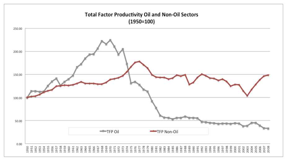
Some authors (Arreaza and Dorta, 2004; Baptista, 2004; Agnani and Iza, 2008) have analyzed TFPs in the Venezuelan oil and non-oil sector, and concluded that the latter is chiefly responsible for the country ́s growth failure.
Looking at the results reported in Table II one is tempted to differ. First, the average annual contribution of TFP for the whole sample period (1950-2008)
turns out to be positive (0.94%) for the non-oil sector, negative (-1.50) for the oil sector. Second, cumulative decline in TFP over the growth-collapse period (1977-2008) totals 10% in the non-oil sector, as compared to 71% in the oil
sector. Moreover, the loss of output per worker in the non-oil sector (-0.70%)
was driven in roughly equal proportions by a decrease in the stock of nonresidential capital per worker (0.31%) and a decrease in total factor productivity (-0.36%); whereas the fall of output per worker in the oil sector (-3.19% per year) occurred in spite of an increase in capital per worker (0.74%), neatly driven by a large decrease in TFPs (-3.19%).
In any case, the fact that the oil sector is an enclave with little forward or backward linkages to the rest of the economy does merit a differential treatment. Oil provides an average of 85% of exports throughout the sample while representing a mere 1.1% of employment. It does not respond to freemarket dynamics: Since 1976 the industry has been managed by the public sector in and its output has been highly restricted by the decisions taken in OPEC. 8 Therefore, any attempt to understand the business cycles in Venezuela will likely benefit from adjusting the calibration to the non-oil economy, fed by oil-driven exogenous shocks.
3. Stylized Facts of the Venezuelan Business Cycle
We have calculated a number of relevant business cycle statistics for Venezuela and the benchmark case of the United States using HP-filtered annual series for the period 1950-2008. 9 10 All series are expressed in logs
(with the exception of the rental rate) and in real terms. The purpose is to get acquainted with the particularities of the business cycle in Venezuela, while providing a benchmark to gauge the effectiveness of RBC model in replicating actual data. The calibration for the latter follows the same guidelines and yields similar results obtained by King and Rebelo (2000) for 1948-1997 using quarterly data.
Venezuela Most of the data used come from the national accounts of the Venezuelan Central Bank and Baptista (2011). The only statistic from a different source is average hours per worker, which was taken from the Total Economy Database of the University of Groningen. As Venezuela lacks a fully functioning and representative stock market, estimates for the annual rental rate have been obtained by dividing the share of output going to capital into the stock of non-residential capital. This ex-post indicator has at least two shortcomings that have been pointed out in the literature. First, given that the rental rate is determined ex-ante, this approach does not incorporate the effects of expectations (Stock and Watson, 1998). Second, using the capital’s share of output results in implausibly high returns on physical capital (Bergoing et.al. 2002). We may neglect the latter, since our interest here does not involve levels but rather cyclical variations. As for the former, it is not so much a matter of convenience but rather one of availability. Results are reported in Table III.
Table III Real Business Cycle Statistics for the Venezuelan Economy
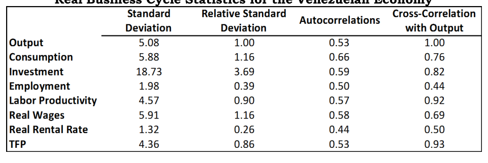
The first and second columns contain absolute and relative volatilities, with the volatility of the cyclical component of output being the reference variable. The volatility of TFP shocks (standard deviation 4.36) is amplified at the level of investment (18.73), real wages (5.91), consumption (5.88), output (5.08), and labor productivity (4.57). In contrast, cyclical variations on the rental rate (1.32) and most notably employment (1.98), are significantly lower and do not amplify TFP shocks.
Most of the remaining figures on Table III are reasonable (i.e. investment much more volatile than output, rental rates much less), so we will focus on two noteworthy and exceptional facts. Having consumption more volatile than output (relative standard deviation 1.16) goes against all economic rationality.
One would expect that had consumers decided not to smooth consumption at all (either for undesirability, lack of financial depth, or a combination), the worst scenario possible would be having consumption equally volatile than output. But it is hard to imagine why rational agents would have their
consumption fluctuating more than output. We would get back to this once we analyze non-oil statistics later on.
The second interesting feature lies on labor markets. The rigidities that prevent the market from adjusting to shocks via quantities (high relative firing costs, widespread minimum salary, and forbidden dismissal below certain salary levels) have driven employment volatility well below that of output (0.39); whilst real salaries display a large relative volatility (1.16). That is to say that extreme restrictions within the labor market have put the burden of adjustment in real salaries, as oppose to quantities, a feature that mirrors well the internal adjustment dynamics of RBC models.
Annual time-series do not display a high degree of persistence, as measured by first order autocorrelations (third column). TFP shocks (0.53) do propagate at the consumption (0.66), investment (0.59), real wages (0.58) and labor productivity (0.57) levels; but not when it comes to output (0.53), employment (0.50) and rental rate (0.44).
At last, most of the time series analyzed tend to move together with the cyclical component of output, as portrayed by the cross-correlations in column four. All variables exhibit pro-cyclical behavior, as they all tend to correlate positively with output, although at different levels of intensity. Labor productivity seems to move together with TFP shocks, both being highly
correlated with output (0.92 and 0.93 respectively). This is also the case of investment (0.82), consumption (0.76), and real wages (0.69). The only variables without significant correlation to output are the rental rate of capital (0.50) and employment (0.44).
Venezuela Non-Oil In order to evaluate the cyclical impact of oil shocks in the non-oil economy we have carved out differentiated business cycle statistics using HPfiltered data. The main interest here lies in analyzing the cyclical variations of the non-oil sector of the economy, given the fact that oil output is governed by factors different from market forces. Data for oil and non-oil output, investment, salaries, employment, and real wages have been obtained from national accounts and Baptista (2011). TFPs have been derived following the standard procedure, using the capital share of output reported by Baptista (2011) in the absence of oil rents (33.9%). Rental rates were estimated as nonoil capital share of output divided into non-oil non-residential capital stock.
In order to replicate Table III for the non-oil economy we have made three assumptions. First, average hours per worker are assumed to be similar in both sectors (since The University of Groningen does not report average hours worked per sector). Second, all oil net investment is assumed to be nonresidential (neither Baptista nor the Central Bank report differentiated residential investment). Third, consumption per unit of labor has been
estimated using total consumption. I believe these assumptions are plausible, if we take into account that we are not dealing here with levels but rather cyclical variations of HP-filtered data.
Real business cycle statistics estimated in such a way will portray a nonresource-abundant economy subject to oil-driven TFP shocks. Such an economy is much more likely to be resembled by RBC theory. Results are reported in Table IV.
Table IV Real Business Cycle Statistics for the Venezuelan Non-Oil Economy
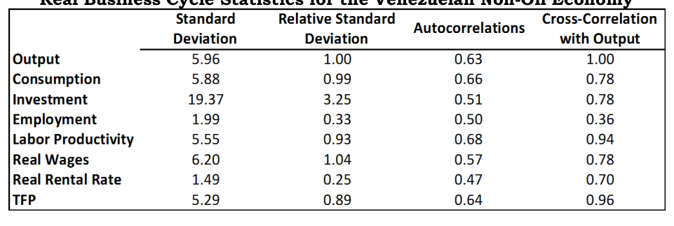
The standard deviation is higher for all the variables selected, with the notable exception of employment, which remained unchanged (1.98 for the economy as a whole, 1.99 for the non-oil sector) 11 . This seems to reinforce the fact that stringent labor legislation affects both sectors alike. Relative volatilities are also quite similar, but a noteworthy feature shows up in the non-oil economy: The cyclical component of consumption is now lower than
that of output. Although the figure is still high (0.99) and points out to little or no smoothing consumption within the non-oil sector, the reduction turns out to be significant (came down from 1.16 to 0.99).
One possible explanation is that total GDP is a composite of a highly volatile non-oil output and a relatively steady oil production. Such an economy is subject to shocks coming from large cyclical swings in oil prices, which impact the demand-side of the non-oil economy (as gathered by the Solow residuals) but are squeezed out of the system without exerting much of a multiplying effect (i.e. via capital flight).
Looking at auto-correlations (column three on Table IV) we can notice that persistence and propagation within the non-oil sector are weaker than in the case for the whole economy. TFP shocks (0.64) only propagate at the level of labor productivity (0.68) and consumption (0.66). All non-oil variables turn out to be pro-cyclical (column four) with coefficients very similar to those reported in Table III.
United States We have calculated a similar set of real business cycle statistics for the benchmark case of the United States. As in the case of Venezuela, all series are expressed in logs (with the exception of the rental rate) and in real terms. All time series have been obtained from the Federal Reserve Bank of Saint Louis
and have been expressed either in constant US $2009 dollars (output, consumption, investment) or in 2009-based real indexes (total hours, wages).
Total hours and wages have been approximated by total hours in the non-farm business sector, as reported also by the Federal Reserve Bank of Saint Louis. I have run the calculations using different index years for the same labor aggregates calculated by the Bureau of Labor Statistics and found no significant difference on the set of selected second moments. The rental rate comes from the annual deflated return of the S&P500 index. Summary statistics for the selected real business cycle variables are reported on Table V.
Table V Real Business Cycle Statistics for the United States (Cyclical variations in real returns using S&P500 as a proxy for rental rate)
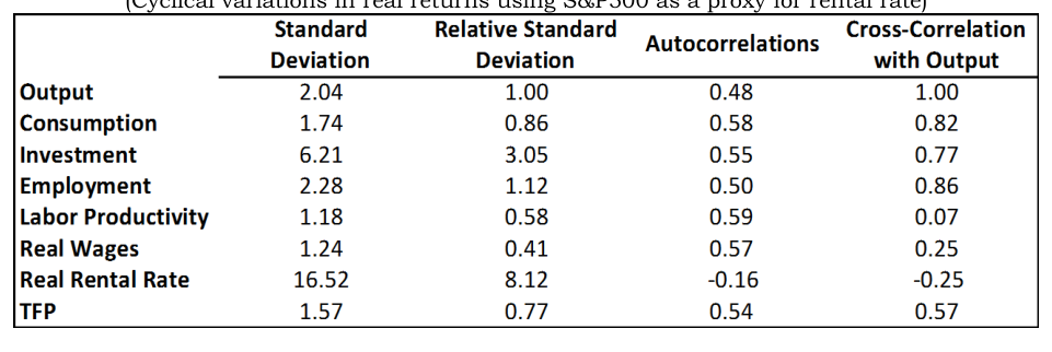
A comparison between standard deviation statistics provides some preliminary insights. Output, consumption, investment, labor productivity and TFPs, unsurprisingly, display a much lower volatility that ranges between a third and a half of that registered in Venezuela for the same aggregates. On the labor market, however, the differences are striking. Average volatility of
employment in the United States is 1.2 times that of Venezuela, while real wages’ one is just 0.2. The large volatility displayed by the rental rate can be attributed to the indicator used (cyclical component of real S&P500 returns) 12 .
We shall get back to this later. By comparing standard deviations on column one of Table V we can also verify that TFP shocks (1.57) amplify to output (2.04), consumption (1.74), investment (6.21), employment (2.28) and rental rate (16.52), except for labor productivity (1.18) and real wages (1.24).
All relative volatilities, autocorrelations and cross-correlations are aligned with those obtained by King and Rebelo (2000) using quarterly data for the period 1947-1996. The cyclical component of consumption is less volatile than output (0.86), whilst investment turns out to be three times as volatile as output (3.05). Employment comes out as more volatile than output (1.12), as opposed to labor productivity (0.58) and wages (0.41).
All auto-correlations are in the order of 0.45-0.60, with the sole exception of rental rate, whose cyclical component displays negative auto-correlation (-0.16) 13 . TFP shock propagation is weak, with all the correlations in the vicinity of the one registered by TFP shocks (0.54). Most of the variables are pro-cyclical, with employment (0.86), consumption (0.82), investment (0.77)
and TFP shocks (0.57) being the ones most correlated with output. Real wages
(0.25) and labor productivity (0.08) display low correlations to output, with the latter very close to being acyclic.
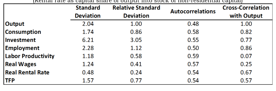
The counter-cyclicality of rental rate of capital (-0.25) in the United States has already been mentioned in the literature and remains a puzzle nowadays, in spite of the numerous efforts to reconcile this with the theory of business cycles (see Kydland and Prescott, 1990; Cooley, 1995; Mertens, 2005; Di Cecio, 2005; and Mertens, 2010). Using the cyclical component of S&P500 returns as a proxy results in a highly volatile and negatively auto-correlated rental rate, two unlikely features of the marginal product of capital we are trying to mirror. In order to ease the comparisons between cycle moments in these two countries we have re-estimated Table V using a proxy for the rental rate obtained in a similar way than in the case of Venezuela: Capital share of output divided into the stock of non-residential capital. As can be seen in Table VI, such a procedure results in rental rates that co-move along with output, similar to Venezuela, although the correlation is lower (0.25 vs. 0.70).
Table VI Real Business Cycle Statistics for the United States (Rental rate as capital share of output into stock of non-residential capital)
4. Standard RBC Model
In this section we outline the formulation and equilibrium conditions of a standard frictionless RBC model.
Preferences, Endowment and Technology There are only two representative agents: households and firms.
Households consume, save (by investing in capital and renting it to firms) and supply labor. Firms produce only one good by combining capital and labor.
The economy is populated by a large number of identical and infinitely lived agents who maximize expected utility given by:
EE 0 ββ tt uu(cc tt , ll tt ) , (3)
where ββ denotes the discount factor, c t is consumption and l t represents leisure. We assume the standard properties of the utility function hold: utility is increasing in both arguments, jointly concave in consumption and leisure, and satisfies the Inada conditions.
Endowments Individuals’ main endowment is time, which can be split into hours of work ( n t ) and leisure ( l t ). For simplicity, the total amount of time is normalized to one, which yields the following time constraint:

Given that for simplicity we are using the most rudimentary version of the neoclassical model (closed economy, no government), all output must be either consumed or invested domestically, as formalized by the aggregate resource constraint:

Technology The standard unit of output is produced by a large number of identical firms. The representative firm combines capital and labor inputs with constant returns to scale (CRS), according to a standard Cobb-Douglas function:
yy tt = aa tt kk tt

where a t is a random total factor productivity shock whose law of motion follows a mean-zero AR(1) process, in logs:
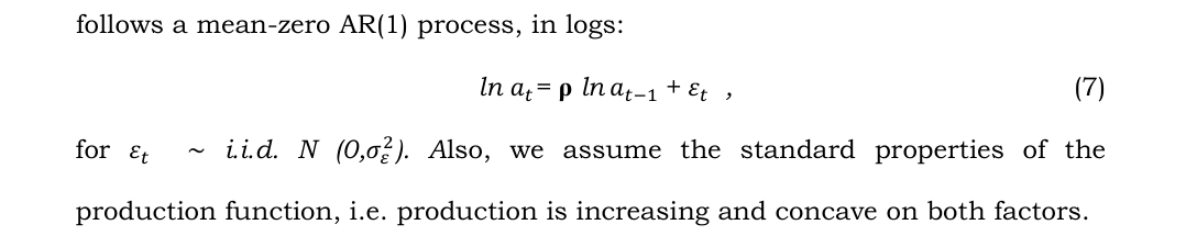
2 ). A lso, we assume the standard properties of the production function, i.e. production is increasing and concave on both factors.
The law of motion of capital stock is then:

where δ denotes the annual depreciation rate.
Based on this formulation, general equilibrium conditions can be computed. The representative household maximizes utility over consumption and leisure subject to his budget constraint and the representative firm
maximizes profits. By equalizing supply and demand for capital and labor we obtain our market clearing prices w t (real wages) and R t (real rental rate of capital).
A representative firm decides how much capital and labor to employ by solving:
max aa tt kk tt

This optimization problem yields real wage and rental rate equations:

and

Given the functional form u (c t , n t ) = ln c t + θθ ln (1-n t ) , the representative household decides how much to consume and supply labor by solving

, (12)
subject to

Equilibrium in this model can be described by a system of non-linear stochastic difference equations and some auxiliary equations:

kk tt+1 = aa tt kk tt

yy tt = aa tt kk tt
5. Calibration

We have calibrated the model’s parameters for the Venezuelan economy (as a whole and for the non-oil sector) and the United States. In most cases the proxies for parameters come from observed long-term features of the timeseries we are modeling. Only in a couple of cases I have relied on highly conventional parameters widely used in the RBC theory for the United States.
The discount factor β was calibrated using the Euler equation for a riskfree bond:
which, when evaluated in steady state 14 , implies:

1+rr (22)
β has been calibrated so that the steady state interest rate coincides with average return to capital. For the case of Venezuela we have used average real returns on capital for the economy as a whole ( r = 13.98% per year ) and the non-oil sector ( r = 9.02% ) as reported in Baptista (2011), which results in β =0.8773 and β =0.9173. For the United States, following the convention of the literature (see Lucas, 1980; Kydland and Prescott, 1982; Long and Plosser, 1983; King and Rebelo, 2000), we computed average real returns on the Standard and Poor 500 Equity Index over the analyzed period (1950-2008); which resulted in r = 6.27%/ year , and β =0.9401.
Average depreciation rate was derived from historical time series data on depreciation expense and capital stock provided by Baptista (2011), resulting in 4.61% per year. Given that there are no records on depreciation by sectors, we have assumed that capital depreciates at the same pace in the oil and nonoil sectors. For the United States we have performed a similar calculation using the data provided by the Federal Reserve Bank of Saint Luois, resulting in yearly depreciation of 5.67%. The latter figure is closed to the one used by Levy (1992, δ = 5.2%), Stokey and Rebelo (1995, δ = 6.0%), and Nadiri and Prucha (1996, δ = 5.9%).
We have used the same capital share on total output for the economy as a whole ( ∝= 0.432) and for the non-oil sector in particular ( ∝= 0.339) that applied in our growth accounting exercise. The latter is reported by Baptista (2011) as
the rate of return on capital excluding oil rents. Baptista (2011) estimates this time serie following a methodology introduced by Baptista and Mommer (1989), consisting in using the rate of return on capital on the non-oil sector of the economy to calculate the rate of return on capital withint the oil sector (the difference being oil rents). For the United States I relied on a parameter ( ∝ = 0.333) widely used elsewhere in the literature.
We calibrated the utility parameter of leisure ( θ ) solving the Euler Equation for the steady state capital-labor ratio:
nn = ቆ , (23)
where we can plug calibrated values for α , β , and δ to calculate the steady state capital-labor ratios. From here, we just need to solve the law of motion of capital for the steady state consumption per worker:
nn = ቀ nn ቁ

nn (24)
Then, we solve the first order condition for labor supply and obtain another expression for consumption per worker:
nn =

nn ቁ (25)
Equating (24) to (25) leads to:
ቀ nn ቁ

nn =

nn ቁ , (26)
and solving for θθ (taking n as given) we obtain:

We have estimated θ so that n matches the long-run average time devoted to work, as reported by the Total Economy Database of the University of Groningen for the United States (21.4%) and Venezuela (22.6%). In order not to have different parameters for leisure between Venezuela and the non-oil sector of its economy, we have used n=0.2258 for the non-oil sector and the standard n=0.20 for Venezuela as a whole. This exercise results in θ =2.90 for the United States and θ =2.68 for both Venezuela and the non-oil sector of the economy. In any case, the results reported below are not contingent on these assumptions, as changes of θ within the [2,4] range do not produce any significant impacts on RBC simulations (see King and Rebelo, 2000).
Finally, we calibrated parameters associated to TFP by using evidence from inside the model. Since this model implicitly assumes that a linear, deterministic trend drives the observed data, we de-trended the TFP series by regressing:

Then we use the estimated residuals uu ො t as a measure of de-trended TFP series and estimate an AR(1) process:

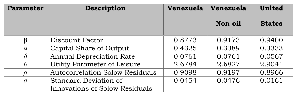
where pp̂ and tt̂ may be taken as proxies for the autocorrelation coefficient of technology and standard deviation of the innovations of Solow residuals. This yields a calibration of pp̂ =0.9098 for Venezuela, pp̂ =0.9197 for the non-oil sector, and pp̂ =0.8966 for the United States. The associated standard deviations are

the United States.
According to these estimations, the persistence of TFP shocks is similar in both countries, but Venezuela turns out to be three times as volatile as the United States. That is precisely one of the shortcomings of the RBC models calibrated for the United States: Shocks are persistent, but they do not exhibit enough volatility as to explain the business cycle (Summers, 1986). And that is where the Venezuelan case, with oil shocks gathered on Solow residuals impacting the non-oil economy, may be a better candidate for RBC predicaments. Table VII summarizes the result from calibration.
Table VII Calibrated Parameters of the Baseline Model
6. RBC-simulated Business Cycle Statistics
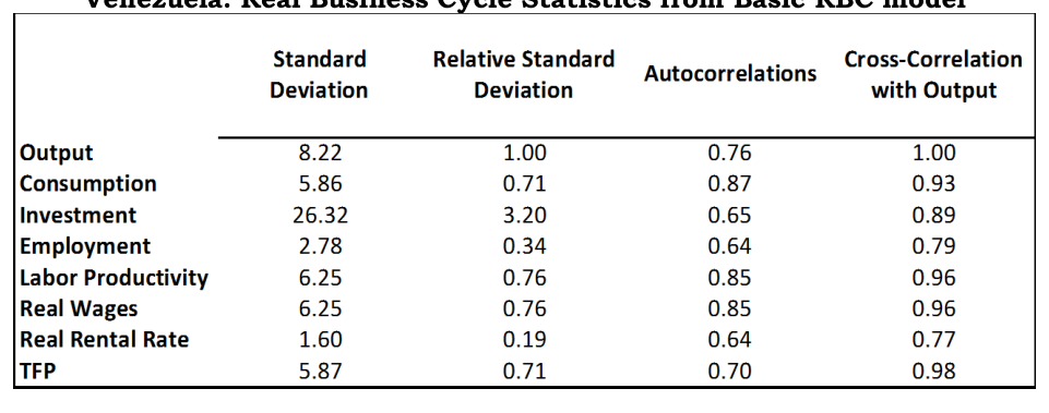
One way to assess the capacity of RBC time series to mirror the actual behavior of the economy during the business cycle is to contrast relevant second moments for simulated and real data. Table VIII below contains standard deviations (absolute and relative), autocorrelations and crosscorrelations with output for a number of real variables, as derived from a RBC standard model calibrated for the Venezuelan economy. We can gather successes and failures by comparing these statistics with those reported on Table III for actual data.
Although the model’s output is more volatile than the actual experience (8.22 vs. 5.08), RBC simulated series does remarkably well in predicting relative volatilities. The model captures the fact that investment is more volatile than output, with simulated relative standard deviation (3.20) coming out relatively close to observed values (3.69). Similar accuracy is registered on relative volatilities of employment (0.34 vs. 0.39), labor productivity (0.77 vs.
0.90), real rental rate (0.19 vs. 0.26) and productivity shocks (0.76 vs. 0.86). As
has been anticipated, the model results on smoothed consumption series that are less volatile than output (0.71), a fact that does not match the awkward feature of real data (1.16). Also, real wages are predicted to be less volatile than output (0.76), when in fact they exhibit a higher relative volatility (1.16).
Modeled volatility of TFP shocks (5.87) is amplified by real wages and labor productivity (6.25), output (8.22) and investment (26.32), a fact that matches well the actual data, where in addition they also amplify to consumption.
As reported in the literature (see Kydland and Prescott 1982 and 1990; King, Plosser and Rebelo, 1998; King and Rebelo, 2000) RBC-simulated time series tend to be more persistent than actual values. The order of autocorrelations goes from 0.64-0.87 in the model, in contrast to 0.44-0.66 in real data. As an immediate consequence propagation is also weaker, with observed TFP auto-correlation (0.53) being slightly below that of productivity (0.57), real wage (0.58), and investment (0.59), when in the model it propagates to all real variables with the sole exception of the rental rate.
RBC rightly predicts all real variables to be highly pro-cyclical. The degree of co-movement with output varies, with predicted cross-correlations for investment (0.89 modeled vs. 0.82 observed), labor productivity (0.96 vs. 0.92)
and TFP shocks (0.98 vs. 0.92) being more accurate than those obtained for consumption (0.93 vs. 0.76), real wages (0.96 vs. 0.69), employment (0.79 vs.
0.44) and rental rates (0.77 vs. 0.50).
Table VIII Venezuela: Real Business Cycle Statistics from Basic RBC model
From this battery of real business cycle statistics we can see that a basic RBC model, one portraying a closed economy without government, produces a surprisingly good account of Venezuela ́s cyclical economic activity. The fit becomes even better if we calibrate the model for the non-oil sector of the economy and contrast its predictions accordingly. Table IX below reports the outcomes of this exercise, which must be compared to Table IV.
Table IX Non-Oil Venezuela: Real Business Cycle Statistics from basic RBC model
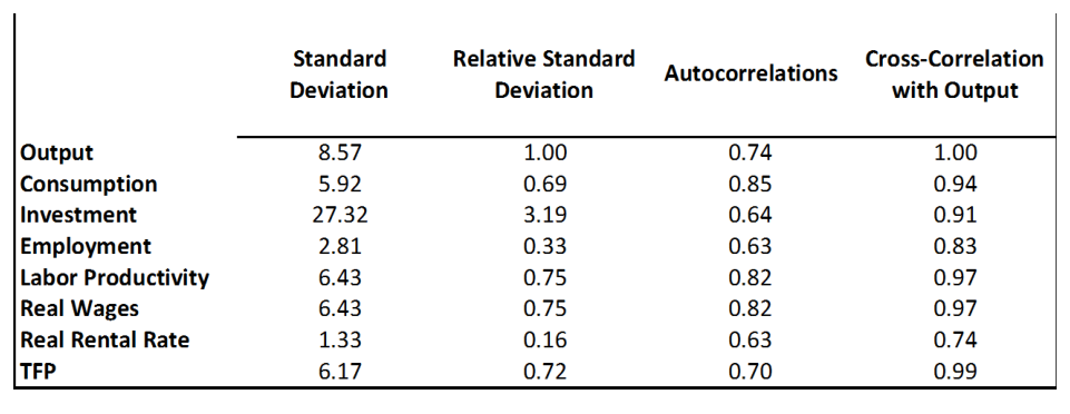
The approximation for the non-oil economy retains all the positive correspondences reported above while improving on certain areas. As expected, the calibration yields output and its components to be more volatile in the nonoil economy, a fact that matches well the actual data (with the exception of consumption, where I have made no distinction between total and non-oil).
As consumption is slightly less volatile than non-oil output (0.99), it resembles better the RBC-simulated relative volatility (0.69). Granted, the simulated value is still lower than the one observed, but this is not an exclusive problem of Venezuela but rather a common feature widely observed in other countries’ calibrations (see section 7 for the benchmark case of the United States). Also, the rank of relative volatilities produced by this approximation matches closely that observed in real variables such as investment (3.19 vs.
3.25), employment (0.33 vs. 0.33); and does well on labor productivity (0.82 vs.
0.93), real wages (0.82 vs. 1.04), TFP shocks (0.70 vs. 0.89) and even rental rate (0.15 vs. 0.25).
7. A rationale for differential RBC performance: Venezuela vs. the
benchmark case of the United States We can contrast the performance of the RBC model in describing the behavior of the Venezuelan economy during the business cycles with the benchmark case of the United States. It is noteworthy that we are opposing one of the most heavily intervened oil-dependent economies in the world with the quintessential fully functioning market, the subject of most of literature empirical applications and adaptations of real business cycle models. To this purpose we have calibrated a basic RBC model for the United States economy and gathered significant statistics on Table X, which we shall compared to the statistics derived from real data as reported in tables V and VI.
Table X United States: Real Business Cycle Statistics from Basic RBC model
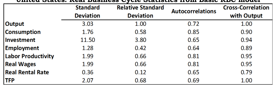
As in the case of Venezuela, modeled output volatility (3.03) is higher than that observed in real data (2.04). The model captures well the fact that investment tends to be more volatile than output (3.80 modeled vs. 3.05
observed). Consumption turns out to be less volatile than output, but the difference between predicted and observed values (0.58 vs. 0.86) is not far from the gap observed in the case of non-oil Venezuela (0.69 vs. 0.99). Persistence and propagation appear stronger in simulated series than in actual data, as well as co-movements with output.
For comparison purposes, given that Venezuela has no representative stock market from which to derive rental rates of capital, we prepared Table VI for the United States. There, we used as a proxy the same statistic as in Venezuela, namely a rate derived from the share of capital in GDP divided into the net stock of non-residential capital. The statistics for the latter are closer to the predictions of the model, either in relative standard deviation (0.12 vs.
0.24), autocorrelation (0.65 vs. 0.54) or cross-correlations with output (0.79 vs.
0.72). More important, the rental rate proxy comes out to be pro-cyclical, just as predicted by the RBC model. The puzzle remains, however, on why stock returns (as reported in Table V) or other expectations-based estimates of the actual rental rate (see Stock and Watson, 1996) come out as anti-cyclical when the ex-post returns on capital as derived from national accounts are consistently pro-cyclical.
The most striking differences are to be found in labor markets behavior.
In the case of the United States, the model predicts a relative standard deviation of unemployment (0.42) that is a third of the value observed in real data (1.12). To the contrary, the model predicts a relative volatility of wages
(0.66) much higher than the one observed (0.41) 15 . One could conjecture that as actual real wages are not as flexible as presumed in the RBC model, the bulk of the adjustment to shocks falls upon quantities (workers).
The opposite happens to be true in Venezuela. Given large restrictions to labor mobility in the form of extremely high firing costs and outright restrictions to outplacements, the bulk of the adjustment to exogenous shocks falls upon prices (real salaries), as opposed to quantities (workers). Simulated relative volatility of employment, either in general (0.34) or non-oil (0.33), almost matches observed values in either case (0.39 and 0.33 respectively).
Employers simply do not venture into hiring workers in a boom, because they are aware that it will be either impossible or very expensive to fire them in a recession.
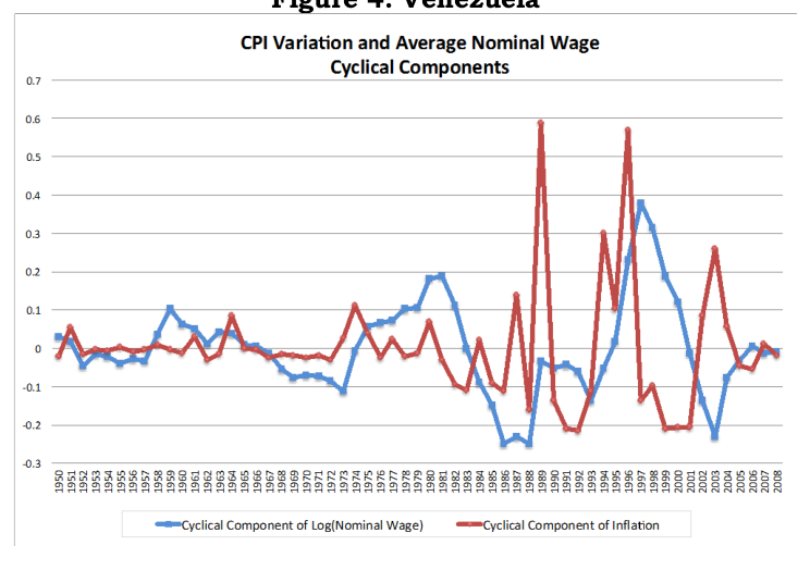
This translates into a highly pro-cyclical real wage, which turns out to be more volatile than presumed in the model, displaying a relative volatility of 1.16 in general and 1.04 in the non-oil economy; a stark contrast with those registered for simulated time series in either case (0.77 and 0.73). The main factor behind the large volatility displayed by real wages is a highly volatile and unpredictable rate of inflation. Figure 4 below contains the cyclical components of the time series for inflation and the log average nominal wages. Although the business cycles have become more pronounced since 1970, the swings in the
cyclical component of inflation have not only out weighted but also preceded those in the average nominal wage, inducing a large volatility in cyclical real wages.
Figure 4: Venezuela
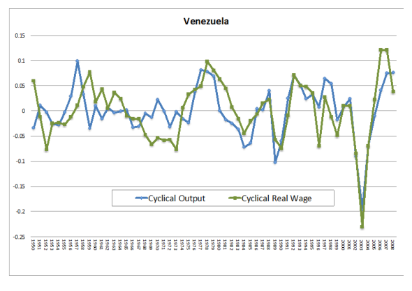
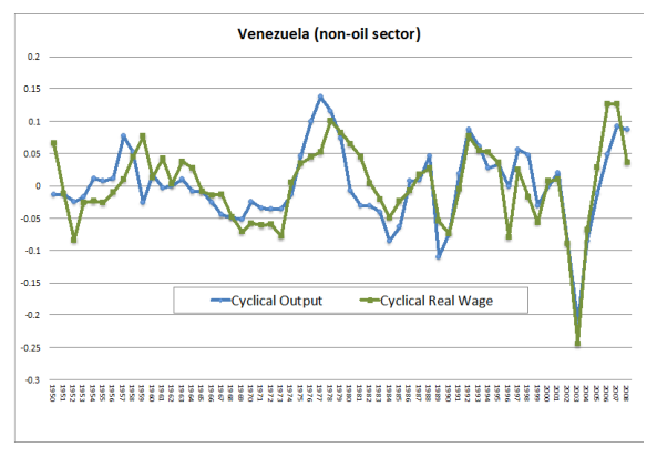
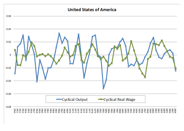
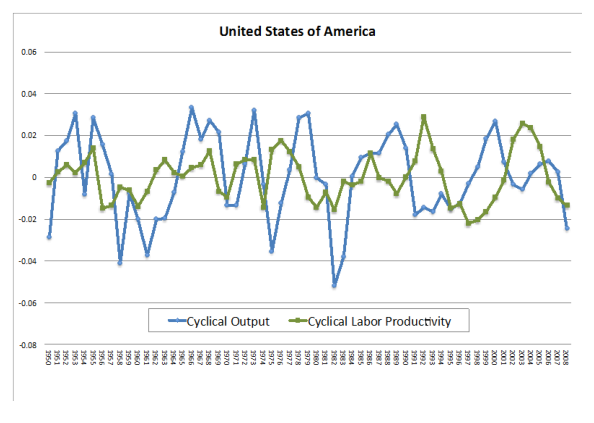
Large differences in the behavior or real wages registered in Venezuela and the United States do mirror the differences in labor productivity. In Figure 5, we report on actual cyclical behavior of real wages and output over 1950- 2008. The correlation in Venezuela is relatively high, either in general (69.1%)
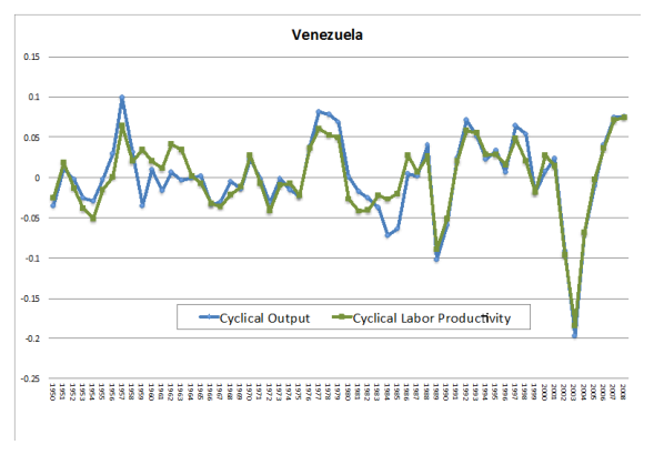
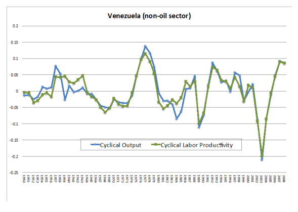
of in the non-oil sector (78.1%). In the United States, to the contrary, observed real wages are much less pro-cyclical, displaying a low correlation with output (24.8%). The disparities between both labor markets in terms of labor productivity are even more salient. As reported in Figure 6, labor productivity displays an almost perfect correlation with cyclical output in Venezuela, either
in general (92.1%) or non-oil sector (94.3%); whereas in the United States there is barely any correspondence (6.7%). Fully flexible real wages and pro-cyclical labor productivity, intrinsic to the mechanics of adjustment of the standard RBC model, are better resembled by the Venezuelan labor market and thereby explain the better fit.
Figure 5 Cyclical Output and Real Wages
8. Conclusions
We have calibrated a standard version of the RBC model to Venezuela and contrasted the accuracy of its predictions to those obtained for the benchmark case of the United States. In spite of being a heavily intervened economy, Venezuela has some particular features that make it appealing from an RBC standpoint. First, growth per capita has remained stagnant over the previous forty years, an unfortunate fact that in turn makes business cycle fluctuations more relevant. Second, the country is subject to large, frequent and highly volatile exogenous shocks, in the form of oil prices. Third, Venezuela has one of the most rigid labor legislations in the world, an arrangement that places all the burden of adjustment to those shocks on real wages.
As it turns out, the calibration of an RBC for Venezuela preserves much of the success registered in the literature for the United States, and performs significantly better on labor markets. Given that oil output does not respond to market forces but is rather decided within the context of a cartel (OPEC), we have also calibrated a standard RBC for the non-oil sector of the economy, which in turn are compared to stylized business cycle facts carved out from national statistics for that sector. The goodness of fit is even better in the latter case, as consumption turns out to be slightly less volatile than non-oil output.
Applying an old free-market framework to a heavily intervened oil-dependent economy provides new insights into both the theory and the country.
From a RBC standpoint, it is surprising that such a strong labor market restrictions are needed to match the predictions of the model. Venezuela is a country where dismissal costs are prohibitive, minimum nominal wage is widespread, and firing employees is forbidden below certain salary thresholds.
And yet, predicted relative volatilities of employment almost exactly match those observed in actual data, either in general or for the non-oil economy. The flip side is real wages that are extremely volatile and highly pro-cyclical, in stark contrast to the sluggishness and lack of correlation with output that real wages exhibit in the United States.
The results reported here reinforce the so-called interest rate puzzle.
Whilst ex-post indicators of returns to capital derived from national accounts do behave pro-cyclically, as predicted by the RBC model, proxies derived from real returns on stock indexes remain anti-cyclical.
For Venezuela, the implications of this paper are far reaching. Protecting jobs by introducing legislation that hinders adjustment in quantities only translates into highly volatile real wages. The net welfare effect of such a policy choice – protecting jobs at the expense of utterly unpredictable real wages – may end up being negative for workers, in particular as liquidity constrains, the only other mean of smoothing out consumption, are all too pervasive in developing countries.
References
• Agnani, B, and Iza, A. (2008). Growth in an oil abundant economy: The case of Venezuela. The Papers 08/18, Department of Economic Theory and Economic History of the University of Granada. • Alayon, A., Daza, A., Carballo, C., Marquez, V. (2002). El costo de la regulacion laboral y de las decisiones judiciales en Venezuela. Edicion UCAB-Conapri, Caracas. • Arreaza, A., and Dorta, M. (2004). Sources of Macroeconomic Fluctuations in Venezuela. Serie de Documentos de Trabajo, BCV, 56. • Baptista, A. And Mommer, B. (1989), Renta petrolera y distribución factorial del ingreso, Instituto Latinoamericano de Investigaciones Sociales (ILDIS), Friedrich Ebert Stiftung, Caracas. • Baptista, A. (2004). El relevo del capitalismo rentístico. Fundación POLAR. • Baptista, A. (2011). Bases cuantitativas de la economía venezolana: 1930- 2008. Fundación POLAR. • Bello, O., Blyde, J., and Restuccia, D. (2011). Venezuela’s growth experience, Latin American Journal of Economics, Vol. 48, No. 2, 199-226. • Bergoing, R. et.al. (2002). A Decade Lost and Found: Mexico and Chile in the 1980s. Review of Economic Dynamics, 5(1), 166-205. • Bosworth, B. and Collins, S. (2008). The empirics of growth: An update, Brookings Papers on Economic Activity 2: 113-179. • Calcavanti, P., de Abreu Pessoa, S., Veloso, F. (2012). On the evolution of TFP in Latin America, Fundacao Getulio Vargas, Instituto Brasilero de Economia (IBRE). • Cole, H., Ohanian, A., Riascos, A., Schmitz Jr., J.A. (2005). Latin America in the rearview mirror, Journal of Monetary Economics, 52: 69-107. • Cooley, T., (1995). Frontiers of BC Research. Thomas Cooley, Editor. 1995. • Di Cecio, R. (2005). Comovement: It is not a puzzle. Working Paper 2005- 035B http://research.stlouisfed.org/wp/2005/2005-035.pdf Federal Reserve Bank of Saint Louis. • Erbil, N. (2011), Is Fiscal Policy Pro-cyclical in Developing Oil Producing Countries?. IMF Working Paper WP/11/171. • Finn, M.G. (1995). Variance properties of Solow’s productivity residual and their cyclical implications. Journal of Economic Dynamics and Control, Volume 19, Issues 5–7, July–September, Pages 1249–1281. • Friedman, M. (1957). A Theory of the Consumption Function, Princeton University Press, Princeton, N.J. • Gertler, Mark & Karadi, Peter, (2011). “A model of unconventional monetary policy,” Journal of Monetary Economics, Elsevier, vol. 58(1), pages 17-34, January. Gertler, Mark, and Nobuhiro Kyiotaki (2011). Financial Intermediation and Credit Policy in Business Cycle Analysis. In Handbook of Monetary Economics, Vol. 3, ed. Benjamin Friedman and Michael Woodford.
• Gollin, D. (2002). Getting income shares right, Journal of Political Economy, 110(2): 458-464. • Gomme, P., and Greenwood, J. (1995). “On the cyclical allocation of risk”, Journal of Economic Dynamics and Control, 19: 91-124. • Hayashi, F., and Prescott,, E. (2002). The 1990s in Japan: A lost decade. Review of Economic Dynamics, 5 (1), January, 206-235. • Hausmann, Ricardo, Talvi, E., Gavin and M., Perotti, R. (1996). Managing Fiscal Policy in Latin America and the Caribbean: Volatility, Pro-cyclicality, and Limited Creditworthiness; Inter-American Development Bank Papers. Inter-American Development Bank Working Paper-326. • Kilian, L. (2006). Not all oil price shocks are alike: Disentangling demand and supply shocks in the crude oil market. CEPR Discussion Paper no. 5994. • King, R., Plosser, C., and Rebelo, S. (1988). Production, growth, and business cycles: I. The basic neoclassical model. Journal of Monetary Economics, 21: 195-232. • King, R., Rebelo, S. (2000). Resuscitating real business cycles, NBER Working Paper No. 7534, February, NBER Program EFG. • Kydland, F., and Prescott, E. (1982). Time to build and aggregate fluctuations. Econometrica, 50: 1345-1370. • Kydland, F., and Prescott, E. (1990). “Business cycles: Real facts and a monetary myth”, Federal Reserve Bank of Minneapolis Quarterly Review, 14: 3-18. • Levy, D. (1994). Capital Stock Depreciation, Tax Rules, and Composition of Aggregate Investment. Journal of Economic and Social Measurement. • Loayza, N., Fajnzylber, P., and Calderon, C. (2005). Economic growth in Latin America and the Caribbean: Stylized facts, explanations and forecasts, Washington DC: The World Bank. • Long, J., and Plosser, C. (1988). Real business cycles. Journal of Political Economy, 91: 39-69. • Lucas, R. (1980). Methods and Problems in Business Cycle Theory. Journal of Money Credit and Banking, 12: 696-715. • Mertens, E. (2005). The Output-Interest Rates Puzzle Conditional on Technology and Monetary Shocks , Study Center Gerzensee and University of Lausanne October. • Mertens, E. (2010). Structural Shocks and the Comovements Between Output and Interest Rates. Finance and Economics Discussion Series Divisions of Research & Statistics and Monetary Affairs, Federal Reserve Board, Washington, D.C. 2010-21. • Nadiri, I. & I. Prucha (1996). Estimation of the Depreciation Rate of Physical and R&D Capital in the U.S. Total Manufacturing Sector. Economic Inquiry (ISSN 0095-2583). Vol. XXXIV, January 1996, 43-56. • Sims, E. (2012). Lecture notes on Graduate Macro Theory II: Stylized Business Cycle Facts and the Quantitative Performance of the RBC Model. University of Notre Dame.
http://www.nd.edu/~esims1/grad_macro_12.html • Stock, J. and Watson, M (1996). Business Cycle Fluctuations in U.S. Macroeconomic Time Series”, in J. Tailor and M. Woodford (eds.) Handbook of Macroeconomics, North-Holland. • Stokey, N. and Rebelo, S., (1995). Growth Effects of Flat-Rate Taxes. Journal of Political Economy, 103: 519-550. • Summers, L. (1986). Some skeptical observations on real business cycle theory. Federal Reserve Bank of Minneapolis, Quarterly Report, Fall 1985, Chapter 5.